Design Rules for 100Mbps Ethernet
| Background.
Now we need to talk about design rules for 100 Mbps or
Fast Ethernet. These networks
have some distinct design constraints due to their speed. The
overall latency for the cables and repeaters combined must meet quite
stringent requirements in order for the network to work properly. For emphasis, the round trip propagation delay table is presented again in this web. The rule is that the delay cannot exceed 512 bit times. The following table summarizes this. |
| Bit Times | Round Trip Propagation Delay | |
10 Mbps Ethernet |
0.1 microseconds | (512)(0.1) = 51.2 microseconds |
100 Mbps Ethernet |
0.01 microseconds | (512)(0.01) = 5.12 microseconds |
| For Fast Ethernet you also need to consider the type of repeaters that are used. The IEEE 100BaseT specification defines two classes of repeaters, Class I and Class II. The following table summarizes their operating characteristics. |
| Delay Time | Hops Allowed | |
Class I |
0.7 microseconds | 1 |
Class II |
0.46 microseconds | 1 or 2 |
| The following table displays the maximum size of collision domains depending on the type of repeater. |
| Copper | Mixed (Copper and Multimode Fiber) |
Multimode Fiber | |
| DTE - DTE | 100 meters | 412 meters 2000 meters (full duplex) |
|
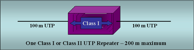
| One Class I Repeater | 200 meters | 260 meters | 272 meters |
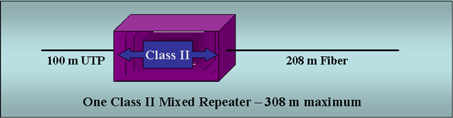
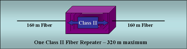
| One Class II Repeater | 200 meters | 308 meters | 320 meters |
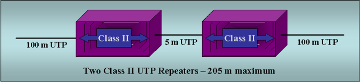
| Two Class II Repeaters | 205 meters | 216 meters | 228 meters |
| But, for example, some Cisco hubs actually perform
better than the standard Class II specifications and then these distances
can be increased. The following images display some of the basic topologies that can be used with different media. There are many others. Remember that UTP refers to unshielded twisted pair. The first diagram can refer to use of either a single Class I or Class II repeater with UTP connectors. |
| The next option makes use of two Class II repeaters over UTP. |
| The next option makes use of a single Class II repeater over a mixture of fiber and UTP. |
| The next option makes use of a single Class II repeater over fiber optic cabling. |
| Let me reiterate that there are many more
configurations that are possible. But it should also be clear that
Fast Ethernet has some definite reach limitations when compared to lower
bandwidth alternatives. Checking the Propagation Delay. To determine whether a particular configuration is valid in terms of propagation delay one needs to make sure they consider all of the following sources of delay.
What are these delays? Answering this question usually depends on some calculations. The following table gives standard delay durations for standard network components. |
| Component Type | Round Trip Delay in Bit Times per Meter | Maximum Round Trip Delay in Bit Times |
| Two TX/FX DTEs | N/A | 100 |
| Two T4 DTEs | N/A | 138 |
| One T4 DTE and One TX/FX DTE | N/A | 127 |
| Category 3 cable | 1.14 | 114 (100 meters) |
| Category 4 cable | 1.14 | 114 (100 meters) |
| Category 5 cable | 1.112 | 111.2 (100 meters) |
| STP cable segment | 1.112 | 111.2 (100 meters) |
| Fiber optic cabling | 1.0 | 412 (412 meters) |
| Class I repeater | N/A | 140 |
| Class II repeater with all TX/FX ports | N/A | 92 |
| Class II repeater with any port T4 | N/A | 67 |
| Making use of these inputs we can outline the steps for determining the delay for any particular path in a collision domain in a network. |
| Step 1 | Determine the delay for each link segment,
denoted LSDV, using the following formula. These computations should
include inter-repeater links. LSDV = 2 x (segment length) x (cable delay for this segment) The 2 makes this a round trip delay. Use cable delay as specified by the manufacturer if reasonable. |
| Step 2 | Add together the LSDVs for all segments in the path |
| Step 3 | Determine the delay for each repeater in
the path. If model specific data is not available from the manufacturer then base this on its class. |
| Step 4 | MII cables for 100BaseT should not exceed
0.5 meters each in length. When evaluating system topology, MII cable lengths need not be accounted for separately. Delays due to MII are incorporated into DTE and repeater delays. |
| Step 5 | Determine the delay for each DTE in the
path. If model specific data is not available from the manufacturer then base this on the above table. |
| Step 6 | Decide on an appropriate safety margin from 0 to 5 bit times. |
| Step 7 | Add together all of these relevant values
to calculate the PDV PDV = link delays + repeater delays + DTE delay + safety margin |
| Step 8 | If the PDV is less than 512 then it is qualified in terms of worst case delays. |
| You can carry out this analysis for all possible paths
in a collision domain in order to get the overall worst case propagation
delay. You may also examine the network for the collision domain and
focus on analyzing the likeliest worst case paths. An Example. Now you need to consider the following example network. |
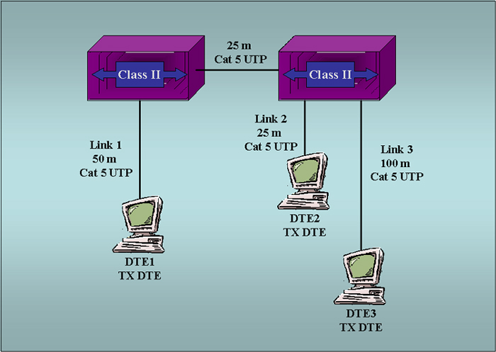
| Notice that we have a non-standard length for the
inter-repeater of 25 meters. This may cause some problems. You
should also notice that we have three paths to consider, though the one
containing Link 1 and Link 3 is clearly longer so we will focus on it as a
worst case scenario. The following table contains the calculations. |
| Cause of Delay | Calculation of Component's Delay | Total (Bit Time) |
| Link 1 | (50 meters)(1.112 Bit Times/meter) | 55.60 |
| Link 3 | (100 meters)(1.112 Bit Times/meter) | 111.20 |
| Inter-repeater link | (25 meters)(1.112 Bit Times/meter) | 27.80 |
| Left Repeater | 92 Bit Times | 92.00 |
| Right Repeater | 92 Bit Times | 92.00 |
| DTE1 and DTE3 | 100 Bit Times | 100.00 |
| Safety Margin | 5 Bit Times | 5.00 |
| Grand Total | Add individual totals | 483.60 |
| So we reasonably make our upper limit of 512 bit times. Since some manufacturers give their propagation delays relative to the speed of light or in nanoseconds per meter you are likely to want to refer to the table on PP129-130 of the Teare book. |