Creating a Pivot Table
Introduction.
PivotTables provide an
interactive way to summarize and present data. It seems that Excel
is the only spreadsheet program that provides this very useful
tool. Using PivotTables gives the user several advatages when they
are implemented.
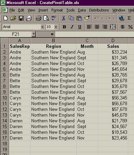
First we will take you through the development of a relatively simple PivotTable and then use this to define a fair amount of terminology. Creating a Pivot Table. Now you should type the following sales data into a new workbook on the first spreadsheet. You only need to format the title row and the sales column at present. Remember you can copy some cells to fill in other cells. |

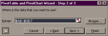
Now you want to invoke the PivotTable Wizard to help
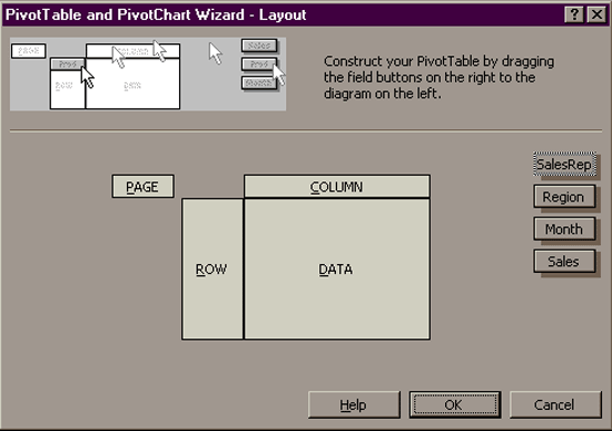
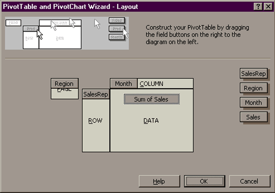
you create the initial PivotTable using the following steps.
|

|
|

|
|
|
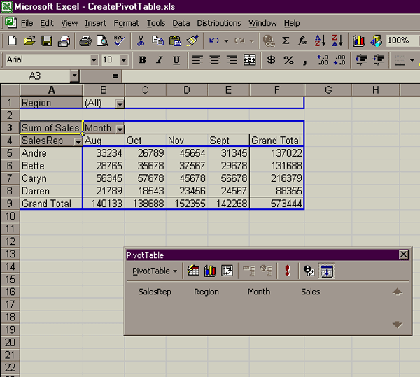
| PivotTable Terminology. The following table contains some jargon that will be defined in terms of the preceding example. |
| Term | Definition | Illustration |
| Row Field | A field with data displayed in rows. | Each SalesRep name is a row field |
| Column Field | A field with data displayed in columns. | Each Month is a column field. |
| Page Field | A field that displays one item at a time. This determines which "page" is displayed in the PivotTable based on the values for the field. | Each Region determines a page where one page shows all regions. |
| Item | A specific row or column heading. | |
| Data Area | The part of the PivotTable where data and calculations are displayed. | The sales figures and the totals. |
Some Quick Modifications.
One of the major advantages of a PivotTable is the ability to change the
view. Let's say, for example, that rather than showing total sales
figures you want to compute averages.
You should see an image like the following. |
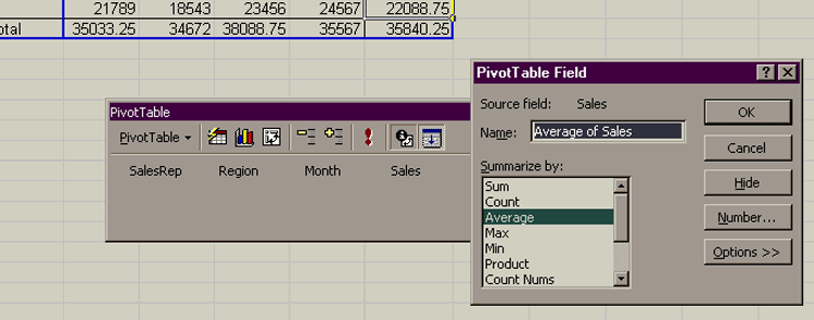
This will change the nature of the calculations. It is obviously easy to change them to many other things. You can easily change the data source range, or the row, column and page fields to quickly get some other informative views. We will leave this to your own exploration. |