Review of Excel Basics Using Mortgages
|
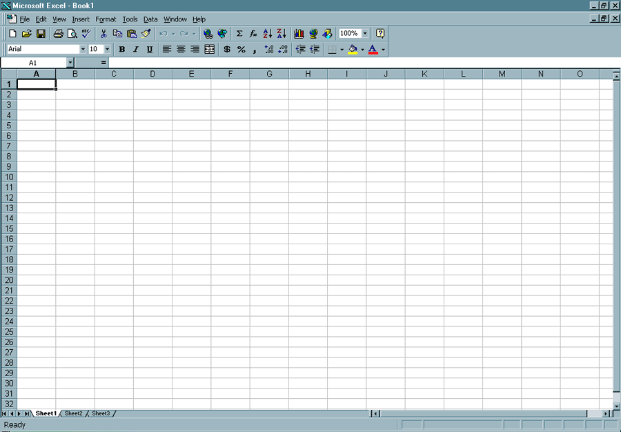
Introduction. By the time you reach college it is likely that you have obtained at least one loan. This may have occurred either to contribute to paying college expenses or buying a car among other things. This sort of situation is very appropriate for reviewing many of the important fundamental features of a spreadsheet program such as Excel. While I am not able to be completely authoritative about the history of spreadsheets, it seems that VisiCalc was the first spreadsheet program for a microcomputer. It was developed by Dan Bricklin and Bob Frankston in 1978 for Apple II computers. It used a row and column based layout and formula syntax that are stilled used today. This evolved through many forms for a variety of platforms. The appearance of Lotus 1-2-3 seems to have helped convince businesses that the IBM-PC was truly a productivity enhancing tool. When Microsoft released Windows 3.0 in 1990, Lotus was slow to get on the bandwagon and didn't quickly develop for the windows user interface. This gave a large opening for Microsoft and they developed Excel. Eventually all the spreadsheet tools migrated to work in a Windows environment along with the Mac-OS. Excel remained one of the major movers. Essentially, a spreadsheet is based on a matrix or array of cells which can hold numbers, text or formulas. One of the most important features of a spreadsheet is the ability to recalculate results as you change the contents of other cells. We will see this feature, along with many others, put to extensive use this semester. Determining Mortgage Payments. You should open your version of Microsoft Excel and you should see a screen that looks a lot like the following. |

|
Notice the cells and the coordinates of each cell using letters for columns and numbers for rows. Now you want to start by typing some text into the cells. We will modify the formats of most of these cells later.
|
| .075 |
| .07625 |
| .0775 |
| .07875 |
| .080 |
| .08125 |
| .0825 |
| .08375 |
| .085 |
| .08625 |
| .0875 |
| .08875 |
| .090 |
| .09125 |
| .0925 |
| .09375 |
|
.095 |
|
| 120000 | 130000 | 140000 | 150000 | 160000 | 170000 | 180000 | 190000 | 200000 |
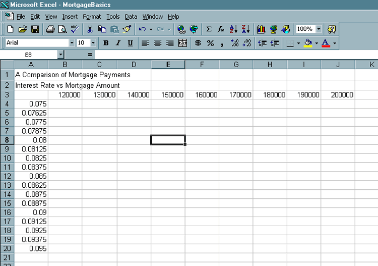
| Now your spreadsheet should look something like the following. |
|
Before proceeding we will format many of the items in the spreadsheet. Some Basic Cell Formatting. It is always worthwhile to make your spreadsheets more readable. You never know who else will see them or whether you will put them down for a while and have to come back to them. You don't want them or you to get lost! The first thing we want to do is put in some sort of legends for the interest rates and the mortgage amounts. This will involve inserting a row and a column and then typing some information into particular cells.
This will insert a new column A.
This should give us sufficient column width for later use.
Now we will put in a legend on the mortgage amounts.
Now we want to format the percentages and dollar amounts so that they are more readable. First the percentages,
Now for the dollar amounts,
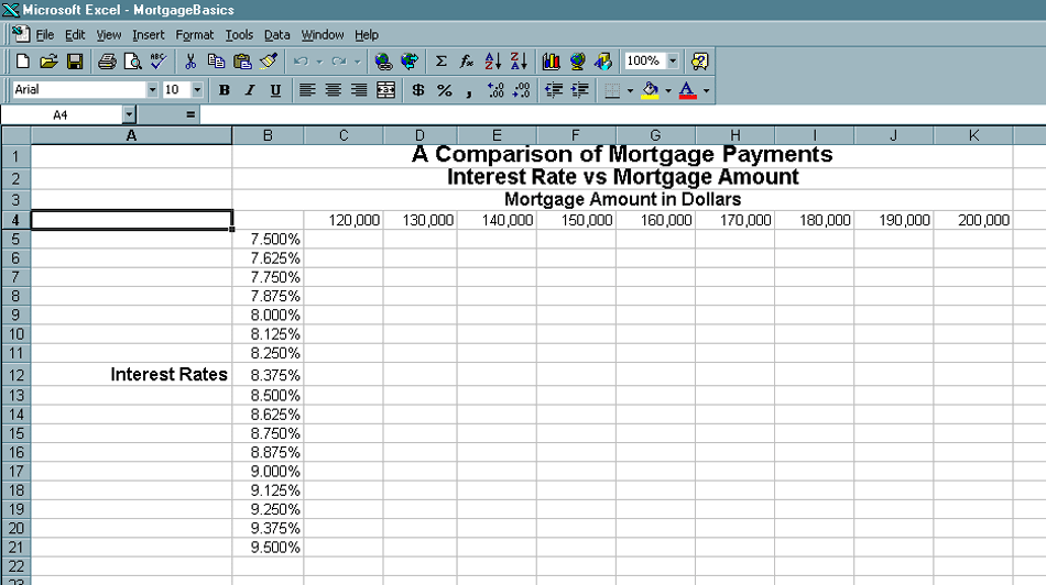
I don't think there is any need to include a dollar sign unless you really would like it. Now your spreadsheet should look like the following. |
|
Before you go any further it is definitely time to save your spreadsheet. Make sure you have a directory/folder for this course. You may want to name it OOPSSVB. Then within this folder you want to have a subdirectory/folder called Mortgages. Click on the save button and save this spreadsheet as MortgageBasics in this Mortgages subfolder. It is extremely important that you organize your examples and homework effectively during this course. If you scatter things around it is difficult to find them and to know what is your most current version. Using Functions. Now we need to fill in the cells within the payments table. Since mortgages are almost always paid using monthly payments this is how we will set this comparison up. I'm quite confident that no one in this room knows the formula for computing these payments off the top of their head. Some of you might not even be able to find it in a book. Computing such values is one of the many advantages of using a spreadsheet since there is a built in function to do the computation. The function is the following. =PMT(rate,nper,pv,fv,type) The meaning of the entries in the function are in the following table. |
| Entry | Description |
| PMT | The function to compute the payments on a loan based on constant payments and a constant interest rate. |
| rate | The interest rate per period of the loan. |
| nper | The total number of payments for the loan. |
| pv | The total amount that a future amount of payments is worth now. In our situation this is just the mortgage amount. |
| fv | The cash balance after all payments have been made. This will default to 0 if omitted. In our situation this is 0. |
| type | 0 or 1 depending on when the payment is made. This defaults to 0 which corresponds to payment at the end of the period. |
|
These entries imply a few things that must be done. Assuming monthly payments
So we need a cell to contain the duration of the loan.
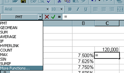
Now we are ready to fill in the payment cells. Fortunately, Excel has some additional help features to make this easier.
|
|
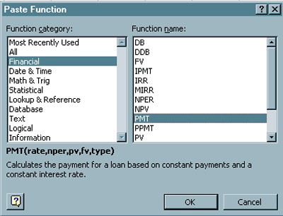
|
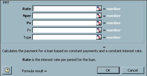
|
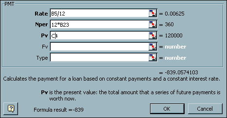
This is telling you that if you get a 30 year mortgage at 7.5% on $120,000 your monthly payments will be $839.06. It is red and in parentheses because it is outgoing money. Copying Cell Formulas. Now that we have gone through all of these steps to develop this cell formula it would be nice if there was some shortcut for filling in the other cells. Fortunately, the people that developed spreadsheets had similar motivation. If you click on the C5 cell you will notice the following formula in the formula bar. =PMT(B5/12,12*B23,C4) Make sure to keep your eye on the cell values as we continue to work. Just for the hyuks, let's copy this formula into the D5 cell and then into the C6 cell. The D5 cell formula becomes =PMT(C5/12,12*C23,D4) The C6 cell formula becomes =PMT(B6/12,12*B24,C5) Notice how when we copy the formula from C5 one cell to the right into D5
In each case the letter also "shifts one to the right" and appropriately becomes C or D. This is due to what is called relative addressing. This is often very convenient. On the other hand notice that when we copy from C5 one cell down to C6 the letters don't change because we stay in the same column, but
In this case the numbers shift down one. The other thing you should notice on your spreadsheet is that you get an error message #DIV/0!. This is because the function is trying to use some argument value that needs to be non-zero. If you change both row and column, both the letters and numbers will change concomitantly. But how can we prevent these adjustments when we want and make desired coordinates not change as we copy? For example, the duration of the loan is always contained in cell B23. We don't want that to change when we copy to other locations. To do this we need to use absolute addressing and put a $ sign in front of each coordinate we don't want to change when we copy. Thus if we are going to copy C5 across the row we want to change the formula to =PMT($B5/12,12*$B$23,C4) so that the percentage rate B5 and the loan duration B15 won't change as we copy across. We want C4 to change to D4 ... K4 as we move across so we don't lock the number and since we are staying in the row we don't have to lock the 4 with a $. If we also want to copy down the column we need to modify the formula to =PMT($B5/12,12*$B$23,C$4) So that we can copy either across or down. After having done this you should get a spreadsheet like the following. |
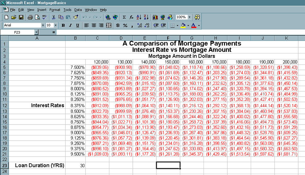
|
Just for the sake of seeing how little the payments increase if you halve the loan duration to 15 YRS you should enter 15 in cell B23 and hit enter to get the sheet to recalculate. Finally, you should right click the tab at the bottom of the sheet that says Sheet1. On the menu that pops up select Rename. Change the name to Payments. Now that you have completed this little exercise we will move on to bigger and better things! |