Some Background.  In the previous webpage we started to work with macros.  The example was largely trivial so that you could focus on the issues associated with creating, cleaning and using macros.  Now I want to develop something more useful that will give you more insight into how a macro might be used in practice.

Consider a new cleaning service called Azulike.  They have been in business for a little over a year and they want to create a computerized approach for developing their Income Statement.  Whether you know it or not the major things an income statement should include are the following.

• Sales figures

• Cost of goods or services sold

• Gross profit

• Fixed costs

• Depreciation expense

• Interest expenses

• Earnings before taxes

• Net income

Recording the Macro.  Now you want to mimic the following steps in order to develop a macro that will format a spreadsheet and set up the cell formulas so that Azulike can more easily develop their income statement for each year.

1. Start by recording a new macro with name IncomeStatementDev.  

2. Give it a shortcut key of Ctrl+i.  

3. Save it in the Personal Macro Workbook so that it will be easily accessible to any other sheet.

4. Highlight cells on cell A1 ... B15.

5. Select the CG Times font and set the font size to 12.  Obviously you can choose another font and size if you want..

6. Type Azulike in cell A1.  Make it bold.

7. Type Income Statement in cell A2.  Make it bold.

8. Type For the Year Ending Dec 31, 2002 in cell A3.  Make it bold.

9. Select cells A1 ... B3.

10. Select the Cells item on the Format menu.

11. Select the Alignment tab.  Select the Center Across Selection in the Horizontal: combo box.

12. Type Sales in cell A5.

13. Type Cost of Goods Sold in cell A6.

14. Type Gross Profit in cell A7.  Make it bold and italic.

15. Type Selling, General and Administrative Expenses in cell A8.

16. Click on the A column header and widen the column so that the entire phrase in cell A8 appears within the cell.

17. Adjust the width of column B to 13.00.

18. Type Fixed Expenses in cell A9.

19. Type Depreciation Expense in cell A10.

20. Type EBIT in cell A11.  Make it bold and italic.  This acronym stands for Earnings before Interest and Taxes.

21. Type Interest Expense in cell A12.

22. Type Earnings Before Taxes in cell A13.  Make it bold and italic.

23. Type Taxes @ 20% in cell A14.

24. Type Net Income in cell A15.  Make it bold and italic.

25. Highlight cells A4 ... B4.  

26. Select the Cells item on the Format menu.

27. Select the Border tab.  Set the upper border line to be a thicker solid line.  Set the lower border line to be a thinner solid line.

28. Select the Patterns tab.  Select a pattern color that you like.  Click on OK.

29. Type 2002 in cell B4.  Make it bold.

30. Highlight cells B5 ... B15.

31. Select the Cells item on the Format menu.

32. Select the Number tab.  Select Number for the Category:.  Select 2 decimal places.  Check the Use 1000s separator checkbox.

33. Select cell B7.  Select the Cells item on the Format menu.

34. Select the Font tab.  Make the font style Bold Italic.

35. Select the Border tab.  Set the upper border to a thin solid line.  Click on OK.

36. Select cell B11.  Select the Cells item on the Format menu.

37. Select the Font tab.  Make the font style Bold Italic.

38. Select the Border tab.  Set the upper border to a thin solid line.  Click on OK.

39. Select cell B13.  Select the Cells item on the Format menu.

40. Select the Font tab.  Make the font style Bold Italic.

41. Select the Border tab.  Set the upper border to a thin solid line.  Click on OK.

42. Select cell B15.  Select the Cells item on the Format menu.

43. Select the Font tab.  Make the font style Bold Italic.

44. Select the Border tab.  Set the upper border to a thin solid line.  Click on OK.

45. Type =B5-B6 in cell B7.

46. Type =B7-Sum(B8:B10) in cell B11.

47. Type = B11-B12 in cell B13.

48. Type =0.2*B13 in cell B14.

49. Type =B13-B14 in cell B15.

50. Stop the recording of the macro.

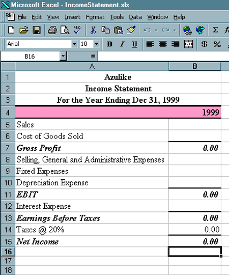
You should now be able to open a new workbook and press Ctrl+i and you will get a template like the following.  At times this may prove to be cumbersome, but you can override this name in any given workbook.  You just can't use the same shortcut key when saving to your Personal Macro Workbook.

Entering Numbers.  Now you want to move to a new sheet and work through the following steps in order to put numbers into the problem.

51. Press Ctrl+i on a new sheet to bring up the template.

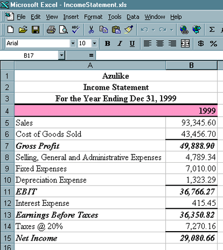
52. Type 93345.60 into cell B5 for the Sales figure.

53. Type 43456.70 into cell B6 for the Cost of Goods Sold, this includes wages.  This will automatically update the Gross Profits figure also.

54. Type 4789.34 into cell B8 for the S, G & A Expenses.

55. Type 7010.00 into cell B9 for the Fixed Expenses.

56. The depreciation expenses are small and estimated to be $1323.29.  Put this in cell B10.  Through all of these steps cell B11 will automatically update.

57. Interest Expense is just $415.45 in cell B12.  Earnings Before Taxes will automatically update in cell B13 as will cell B14 for Taxes.  Finally cell B15 should also automatically update.

Now you should save the file and call it something like IncomeStatement in a separate folder for Azulike.

After entering these numbers the spreadsheet should look like the following.  You will augment this spreadsheet further in the homework to include percentages.