Exponential Smoothing
| Introduction.
Now that I have blabbed and waved my hands about some generalities
associated with forecasting we need to focus on some particular
approaches. The broad name that characterizes our approach is time
series forecasting. A time series essentially means
that you have data over time. For example, you have on-hand
inventory levels for each month, you have sales revenues for each
quarter. Basically you have the past history of a particular
entity of interest, but that is all. This is a relatively minimal,
but entirely common, approach to forecasting.
With time series forecasting you are typically going to try and determine four major things in the data
Since this is a course in CIS and not in Operations the only methods we will examine will focus on trying to find the underlying signal. Think of finding the radio signal using a tuner. What is the basic movement in the data? How can we filter out all the noise and get to the fundamental flow of demand? There are many approaches to doing time series forecasting from something called Box-Jenkins to the Winter's Model. We will work on some of the simplest and most common approaches in this segment of the course. We will start with one of the most common approaches called exponential smoothing. Exponential smoothing can be considered to be an effort to determine the underlying signal. Exponential Smoothing. Now we start developing some background specific to exponential smoothing. One of the main features of exponential smoothing is that it makes use of a weight to determine the influence of observed past values to predict the present.
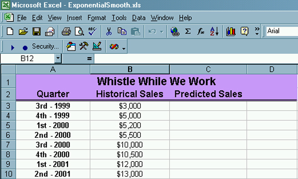
The formula for the present forecast is present forecast = (weight * previous observation) + ((1 - weight) * previous prediction) Well, this is an attempt to put it into words. How this is done in practice is probably best illustrated by an example. Consider a new cleaning company started by your estranged half sister called Whistle While We Work. You have some past sales data represented by the following section from a spreadsheet. |
| Notice how there is some sort of underlying growth
trend in revenues. What we need to do is construct a spreadsheet
like the following.
The formula for cell C4 is =B3 so that your first prediction is just your first observed value. The formula for cell C5 is =$B$13*B4 + ((1-$B$13)*C4) Now you can copy this formula down through cell C11. |
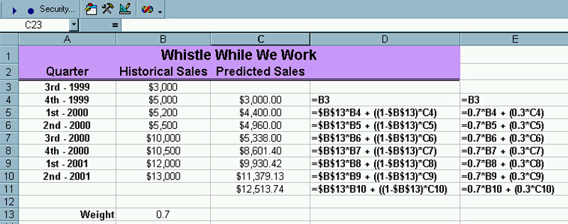
Notice that all of the historical data is used in the
computations.
Even though this will adapt to changes in the entry for cell B13, we eventually want to create a function in order to implement this procedure in even more general situations.
This iteration will carry you one period into the future to give you a prediction. If you graph the historical data and the predictions you get something like the following. |
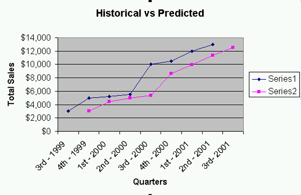
| While it is difficult to tell with this data set, the
graph of the predictions is slightly smoother. You should
definitely look at how these results change as you change the weight
between 0 and 1.
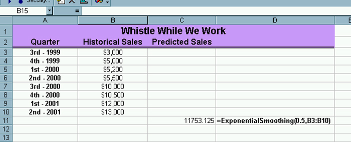
Developing the Exponential Smoothing Function. Now we need to develop the code for the exponential smoothing forecast that can be used more flexibly. The code follows. Notice that the inputs are both the weight and the array of historical values. You can store it in whatever workbook you want. Function
ExponentialSmoothing(Weight, Historical) As Single
Next Item The code will be explained in class. You want to position the function on the spreadsheet so that the result of the computation appears where it should like the following. |