Developing User Functions to Assess Risk in a Stock


Introduction.  In the last two webpages we have talked about risk and returns associated with individual stocks and then with portfolios based on past performance.  Now we will examine estimating risk on future returns in another way.

It is quite typical to use past performance of a stock to develop some sort of distribution to estimate future returns.  We are still going to look at the Stock A and Stock B that we have been working with before.  The following tables estimate the probabilities of particular percentage growth rates in the next year.  We are not going to get into how these probabilities were estimated.


Stock A
Growth Probability
0% 0.1
5% 0.2
10% 0.3
15% 0.3
20% 0.1
Stock B

Growth

Probability
0% 0.05
5% 0.3
10% 0.2
15% 0.2
20% 0.25


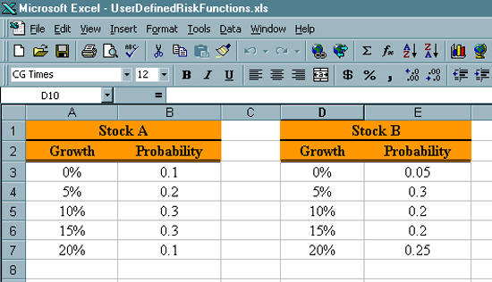
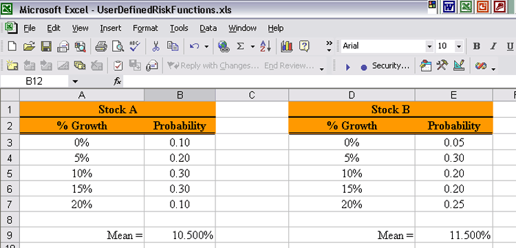
How can we compare the gains we might expect to see for these stocks given this new way of presenting the information? 

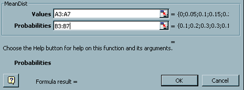
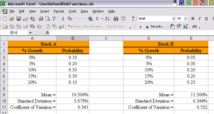
We can think of this new codification as a discrete distribution.  The percentage rate of return is the random variable.  The entries in each of the Growth columns is the potential values of the random variable.  The entries in the Probability column are the probabilities that the growth will be the corresponding value in the Growth column.

But as is always the case it is difficult, if not nearly impossible to compare entire distributions.  Comparisons are more successful if they are done between single numbers.   Again we will work with expectations.  We will again want to use the mean, standard deviation and coefficient of variation.  But Excel does not have any built in functions for these performance measures when we are working with distributions.  The functions we used in the previous webpages related to sample expectations.

The first thing we need to do is refer to a Statistics text to find the formulas for these expectations when we are working with distributions.  Then we will need to develop our own functions for computing these performance measures.

Expectations for Discrete Distributions.  What we are working with in this situation are called discrete distributions.  We will now present the formulas for our desired expectations for discrete distributions.

Consider a random variable X that can take on the discrete values


where


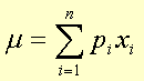
The distribution mean is

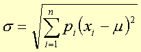
The distribution standard deviation is

The distribution coefficient of variation is


Setting Up the Spreadsheet.  At this point you want to open a new workbook and fill in the cells so that they look like the following.

User Defined Function for the Mean.  Now we need to develop some VisualBasic code to implement the computation of the expectations in a function.  Then we can use these newly developed functions in a spreadsheet just like we use the Excel built in functions.  

Notice that for computation of the mean of the distribution you need to multiply each value times the probability the random variable takes on that value and then add them up.  You can consider the values that the random variable take on to be an array called Values.  You can consider the probabilities that the random variable takes on each of these values to be an array called Probabilities.  Considering this the following code defines a function that will computer the mean for the discrete distribution when used in a cell formula.

Function MeanDist(Values, Probabilities) As Single
Dim Item As Variant
Dim Counter As Integer
MeanDist = 0#
Counter = 1

For Each Item In Values

MeanDist = MeanDist + (Values(Counter) * Probabilities(Counter))
Counter = Counter + 1

Next Item
End Function

We will not go into a lot of detail in this webpage about this code.  We will discuss it in class.  Notice the name of the function is MeanDist for the mean of a distribution.  Since it is a function and it is defined as single it will return a single precision value.  Two arguments need to be passed into the function in order for it to work.  The first argument is an array of the values that the random variable can take on.  The second argument is an array of the probabilities for each value of the random variable.  The value of MeanDist starts out at 0.0 and is then incremented by each value times the probability the random variable will take on that value.  After having looped through each item in the array the summing of the increments is completed.  You should be familiar with the For ... Next loop from your earlier courses.

Now we will implement the function in the UserDefinedRiskFunctions.xls workbook by working through the following steps.

  1. Click on the VisualBasic Editor toolbar button to bring up the IDE.
  2. Insert a new module if necessary.
  3. Copy the above code into the code window.
  4. Go back to the spreadsheet.
  5. Type Mean = in cell A9.  Right justify it.
  6. Type an = sign in cell B9.
  7. Then click on the Functions button to the left of the formula bar, but make sure to click on the downward pointed triangle to bring up the combo box.
  8. Select the More Functions item in the combo box to bring up the following dialogue form.


  1. Scroll in the Function Category: list box and select User Defined.
  2. In your case this should bring up only the MeanDist function in the Function Name: list box.  Select the MeanDist function.
  3. Click on OK.
  4. This will bring up the following function dialog form for the MeanDist function.


  1. Now you can work with this dialogue to fill in the appropriate arrays
    • A3:A7 for Values
    • B3:B7 for Probabilities


  1. Format cell B9 as a Percentage with 3 decimal places are showing.
  2. Copy cells A9 ... B9 to cells D9 ... E9.

Now your spreadsheet should look like the following.

User Defined Function for the Standard Deviation.  Now we want to go through very similar steps to develop the User Defined function for computing the distribution standard deviation.  The following code should be copied into the code window.

Function StdDevDist(Values, Probabilities) As Single
Dim Item As Variant
Dim Mean As Single
Dim Counter As Integer
StdDevDist = 0#
Counter = 1

Mean = MeanDist(Values, Probabilities)

For Each Item In Values


StdDevDist = StdDevDist + (Probabilities(Counter) * (Values(Counter) - Mean) ^ 2)
Counter = Counter + 1


Next Item

StdDevDist = StdDevDist ^ 0.5
End Function

The meaning of the code will be discussed in detail in class.   Notice the name of the function is now StdDevDist for the standard deviation of a distribution.  Since it is a function and it is defined as single it will return a single precision value.  Two arguments need to be passed into the function in order for it to work.  The first argument is an array of the values that the random variable can take on.  The second argument is an array of the probabilities for each value of the random variable.  You need the mean of the distribution in order to compute the standard deviation so the MeanDist function is used to compute the Mean.  The value of StdDevDist starts out at 0.0 and is then incremented by the quantity of each value minus the mean squared times the probability the random variable will take on that value.  After having looped through each item in the array the summing of the increments is completed.  Then since we need the standard deviation we need to take the square root of this sum.

You now want to work through the following steps in order to compute the distribution standard deviations on the stock performance estimates.

  1. Click on the VisualBasic Editor toolbar button to bring up the IDE.
  2. Insert a new module if necessary.
  3. Copy the above code into the code window.
  4. Go back to the spreadsheet.
  5. Type Standard Deviation = in cell A10.  Right justify it and widen the column so that the identifier fits.
  6. Type an = sign in cell B10.
  7. Then click on the Functions button to the left of the formula bar, but make sure to click on the downward pointed triangle to bring up the combo box.
  8. Select the More Functions item in the combo box to bring up the following dialogue form.
  9. Scroll in the Function Category: list box and select User Defined.
  10. In your case this should bring up only the StdDevDist function in the Function Name: list box.  Select the StdDevDist function.
  11. Click on OK.
  12. This will bring up the function dialog form for the StdDevDist function.
  13. Now you can work with this dialogue to fill in the appropriate arrays
    • A3:A7 for Values
    • B3:B7 for Probabilities
  14. Format cell B10 as a Percentage with 3 decimal places are showing.
  15. Copy cells A10 ... B10 to cells D10 ... E10.  Make sure to widen column D enough to contain all of the words.

This will fill in the distribution standard deviations for each stock.  Now we will finish this by developing the function for the distribution coefficient of variation.

Computing the Distribution Coefficient of Variation.  This last computation will go quite quickly considering that the coefficient of variation is formed purely by the mean and standard deviation of the distribution.  The code that should be copied into the code window follows.

Function CVDist(Values, Probabilities) As Single
CVDist = StdDevDist(Values, Probabilities) / MeanDist(Values, Probabilities)
End Function

You want to work through the following steps.

  1. Click on the VisualBasic Editor toolbar button to bring up the IDE.
  2. Insert a new module if necessary.
  3. Copy the above code into the code window.
  4. Go back to the spreadsheet.
  5. Type Coefficient of Variation = in cell A11.  Right justify it and widen the column so that the identifier fits.
  6. Type an = sign in cell B11.
  7. Then click on the Functions button to the left of the formula bar, but make sure to click on the downward pointed triangle to bring up the combo box.
  8. Select the More Functions item in the combo box to bring up the following dialogue form.
  9. Scroll in the Function Category: list box and select User Defined.
  10. In your case this should bring up only the StdDevDist function in the Function Name: list box.  Select the CVDist function.
  11. Click on OK.
  12. This will bring up the function dialog form for the CVDist function.
  13. Now you can work with this dialogue to fill in the appropriate arrays
    • A3:A7 for Values
    • B3:B7 for Probabilities
  14. Format cell B11 as a Number with 3 decimal places showing.
  15. Copy cells A11 ... B11 to cells D11 ... E11.  Make sure to widen column D enough to contain all of the words.

Now your spreadsheet should look like the following.

The last thing to consider is all of the things that could go wrong when inputting the values for computing the functions.  It is important to be able to make sure that the inputs have at least certain levels of validity.  These issues will be taken up in the next webpage.