Assessing Long Term Stock Risk Using Excel
|
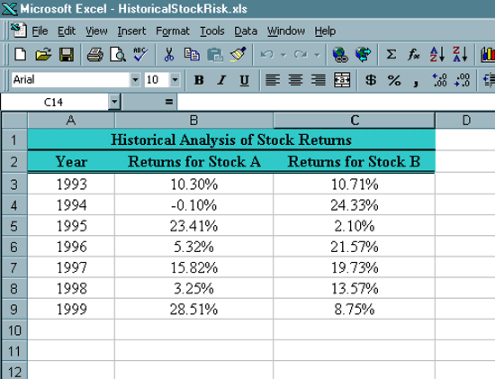
Introduction. Let's assume you have a couple thousand dollars and you are looking to purchase stock in at least a couple different corporations. You are expecting to hold onto this stock for a fairly long time. You are not a day trader. You know a fair amount about two different companies based on past experience and you are curious about their stock performance. The first step is to collect some information on the annual percentage gains for two different stocks over the last several years. The desired information is contained in the following table. |
| Year | Returns for Stock A | Returns for Stock B |
| 1993 | 10.30% | 10.71% |
| 1994 | -0.10% | 24.33% |
| 1995 | 23.41% | 2.10% |
| 1996 | 5.32% | 21.57% |
| 1997 | 15.82% | 19.73% |
| 1998 | 3.25% | 13.57% |
| 1999 | 28.51% | 8.75% |
|
Notice that both of these stocks have had some very good years along with some off years. You are likely to want to find some sort of average rate of return, but you are also going to be concerned with the variation in returns. Now you want to start by typing some text into the cells. We will modify the formats of most of these cells later.
At this point your spreadsheet should look like the following. |

| Computing Expectations.
The word expectations has considerable statistical meaning in addition
to its typical usage. We will compute measures that are averages of the values or averages of the dispersion or some ratios of
these measures. Expectations are used to give single measures that
somehow represent the data they are derived from. It is not easy
to make decisions based on an entire distribution, but it is much easier
to describe expectations about the mean or dispersion. While a
decision maker definitely loses information by creating these
expectations they still provide a lot of usefulness.
The first expectation we will work with is called the mean. This should be quite familiar. The definition of a sample mean is
where is the sample. But as you can see the mean is not a perfect representation of the overall distribution. For example, using the average height and size of everyone to make clothes all the same size would not be very effective. Yet by the same token the mean does give some information about the distribution of data, at least a general sense of its center of gravity. Another feature of a distribution of data is the extent to which it is spread out. There are several measures that are typically used to represent this, such as the range and variance. We will focus on the standard deviation since this has the same units as the data. The definition of the sample standard deviation for the same sample as above is
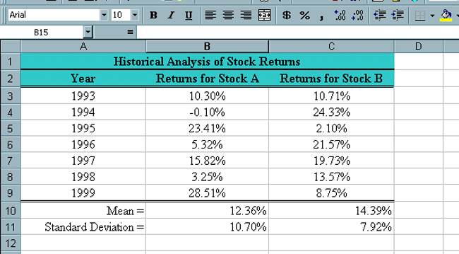
Now you should compute the mean and standard deviation for the stock data.
Now the spreadsheet should look like the following. |

| Notice that they each have different means and standard
deviations. In this case Stock B does better with both
measures. This is seldom the case.
The greater the standard deviation of such returns the greater the risk of investing in the stock. There is one other measure we want to consider called the coefficient of variation. It is often the case that something with a larger mean will also have a larger standard deviation. Consider
If you were going to try and compare the variation between them you would find that the standard deviation of the heights of the people is much greater than the standard deviations of the lengths of the pencils. But sometimes it is important to try to compare the amount of variation between seemingly disparate things such as the price of Microsoft and the price of an IPO. They are almost surely going to appear on very different scales. But if we divide the standard deviation associated with each of the stocks by their respective means we are much more likely to get a ratio that we can compare. The sample coefficient of variation is defined as
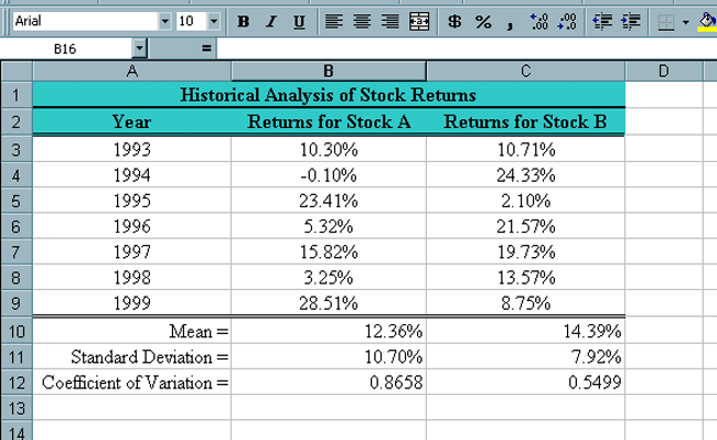
Excel does not have built in function for CV, but we can easily compute them with the following steps.
You should now have a spreadsheet like the following. |

| Notice that the coefficient of variation for Stock B is
also better.
At present it might appear that you should put all of your money into Stock B since it has the higher mean growth rate and the lower standard deviation. In spite of this there are reasons for continuing to consider purchasing quantities of both stocks. In the next web page we will use Excel to investigate putting stocks together into a portfolio to improve returns and decrease risk. |